🔭 Using the GaiaUnlimited precomputed APOGEE selection function#
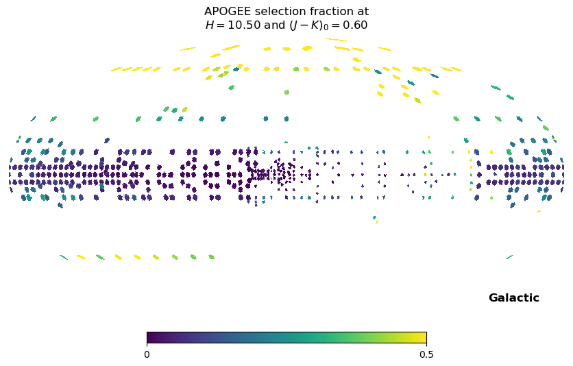
The APOGEE selection function depends on the apparent magnitude of the source in the \(H\) band, on its intrinsic colour (because the APOGEE target selection is performed on de-reddened photometry) and on the location on the sky.
The gaiaunlimited package provides the function gaiaunlimited.apogee_sf which takes three arguments: the apparent magnitude \(H\), the intrinsic colour \((J-K)_0\), and the location on the sky (as an astropy coordinate object).
import gaiaunlimited
from gaiaunlimited import utils
import numpy as np
import matplotlib.pyplot as plt
Warning: the passwords of all user accounts have been inactivated. Please visit https://cas.cosmos.esa.int/cas/passwd to set a new one. Workaround solutions for the Gaia Archive issues following the infrastructure upgrade: https://www.cosmos.esa.int/web/gaia/news#WorkaroundArchive
For this example I map the entire sky in healpix regions of order 7 to make the end figure look nicer. It takes several minutes to complete. Using healpix_order=4 only takes a few seconds.
%%time

healpix_order = 7

H_to_query = 10.5
JK0_to_query = 0.6

# Grab the coordinates of the centres of healpix regions:
coords_of_centers = utils.get_healpix_centers(healpix_order)
NNN = len( coords_of_centers )

# Query the precomputed selection at those locations:
sel_frac_apogee = gaiaunlimited.apogee_sf(H_to_query*np.ones(NNN),JK0_to_query*np.ones(NNN),coords_of_centers)
sel_frac_apogee = np.array(sel_frac_apogee)
sel_frac_apogee[ sel_frac_apogee==0 ] = np.nan
CPU times: user 2min 47s, sys: 5.65 ms, total: 2min 47s
Wall time: 2min 47s
import healpy as hp

hp.mollview(
    sel_frac_apogee,
    nest=False,
    coord="CG",
    min=0,
    max=0.5,
    title="APOGEE selection fraction at\n$H=%.2f$ and $(J-K)_0=%.2f$"
    % (H_to_query, JK0_to_query),
    badcolor="white",
)
plt.show()
How we constructed the APOGEE selection function#
The method we followed to obtain the APOGEE selection function was introduced in Bovy et al. (2014) (see also Bovy et al. (2016) and Frankel et al. (2019)).
The idea is: in each field observed by APOGEE, count the number of 2MASS targets in bins of \(H\) and \((J-K)_0\), then count which fraction of them have corresponding APOGEE data.
from astropy.table import Table
import matplotlib.pyplot as plt
import numpy as np
Read the table containing stellar parameters for APOGEE DR17#
NOTE For this to work you need to download the allStarLite table locally, the file is about 1.8 GB:
https://www.sdss4.org/dr17/irspec/spectro_data/.
Also modify the path in the next line of code.
from astropy.table import Table

tAllstars = Table.read(
    "/home/brown/Gaia/GaiaUnlimited/APOGEE/allStarLite-dr17-synspec_rev1.fits"
)
WARNING: hdu= was not specified but multiple tables are present, reading in first available table (hdu=1) [astropy.io.fits.connect]
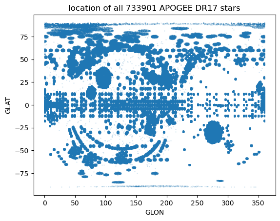
plt.scatter(tAllstars["GLON"], tAllstars["GLAT"], s=1, alpha=0.1)
plt.xlabel("GLON")
plt.ylabel("GLAT")
plt.title("location of all %i APOGEE DR17 stars" % (len(tAllstars)))
Text(0.5, 1.0, 'location of all 733901 APOGEE DR17 stars')
%%time
fieldsWeWant = []
for i in range(len(tAllstars)):
    if tAllstars['PROGRAMNAME'][i] in ['bulge','disk','disk1','disk2','apogee']:
        try:
            a = int(tAllstars['FIELD'][i].split('+')[0])
            b = int(tAllstars['FIELD'][i].split('+')[1])
            c = a+b
            fieldsWeWant.append( tAllstars['FIELD'][i] )
        except:
            try:
                a = int(tAllstars['FIELD'][i].split('-')[0])
                b = int(tAllstars['FIELD'][i].split('-')[1])
                c = a+b
                fieldsWeWant.append( tAllstars['FIELD'][i] )
            except:
                pass


fieldsWeWant = sorted(set(fieldsWeWant))
print('We have retained %i fields.' % (len(fieldsWeWant)))
We have retained 566 fields.
CPU times: user 6.45 s, sys: 7 ms, total: 6.46 s
Wall time: 6.47 s
We only want stars that belong to grid pointings. They have:
a PROGRAMNAME = ‘bulge’, or ‘disk’, or ‘disk1’, or ‘disk2’, or ‘apogee’
a FIELD name indicating it is a grid pointing, i.e. “LLL+BB” or “LLL-BB”
Read the table describing the design of all APOGEE and APOGEE-2 pointings#
This table is a much smaller file than the entire APOGEE DR17 data, so we read it directly from the website:
target_url = "https://data.sdss.org/sas/dr17/apogee/target/allDesign.fits"
tDesigns = Table.read(target_url)
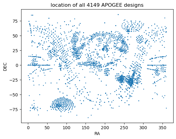
plt.scatter(tDesigns["RA"], tDesigns["DEC"], s=1)
plt.xlabel("RA")
plt.ylabel("DEC")
plt.title("location of all %i APOGEE designs" % (len(tDesigns)))
Text(0.5, 1.0, 'location of all 4149 APOGEE designs')
If a given field was targeted with more than one design, verify that the design was the same every time, or else the selection function is not tractable. The values of:
COHORT_MIN_H
COHORT_MAX_H
BIN_DEREDDENED_MIN_JK_COLOR
BIN_DEREDDENED_MAX_JK_COLOR
RADIUS
LOCATION_ID
must remain unchanged for repeated designs of a given field.
# remove trailing spaces in field names:
designFieldNames = np.array([n.strip() for n in tDesigns["FIELD_NAME"]])
inconsistentField = [] # for all fields with inconistent designs
for j, f in enumerate(fieldsWeWant):
reduced_tDesigns = tDesigns[
"COHORT_MIN_H",
"COHORT_MAX_H",
"BIN_DEREDDENED_MIN_JK_COLOR",
"BIN_DEREDDENED_MAX_JK_COLOR",
"RADIUS",
"LOCATION_ID",
]
reduced_tDesigns = reduced_tDesigns[designFieldNames == f]
# if more than one row in reduced_t, check that they are all the same:
if len(reduced_tDesigns) > 1:
for ii in range(len(reduced_tDesigns)):
if reduced_tDesigns[0]["RADIUS"] != reduced_tDesigns[ii]["RADIUS"]:
# print(f,reduced_tDesigns)
inconsistentField.append(f)
break
if (
reduced_tDesigns[0]["LOCATION_ID"]
!= reduced_tDesigns[ii]["LOCATION_ID"]
):
# print(f,reduced_tDesigns)
inconsistentField.append(f)
break
if np.any(
~(
reduced_tDesigns[0]["BIN_DEREDDENED_MIN_JK_COLOR"]
== reduced_tDesigns[ii]["BIN_DEREDDENED_MIN_JK_COLOR"]
)
):
# print(f,reduced_tDesigns)
inconsistentField.append(f)
break
if np.any(
~(
reduced_tDesigns[0]["BIN_DEREDDENED_MAX_JK_COLOR"]
== reduced_tDesigns[ii]["BIN_DEREDDENED_MAX_JK_COLOR"]
)
):
# print(f,reduced_tDesigns)
inconsistentField.append(f)
break
if np.any(
~(
reduced_tDesigns[0]["COHORT_MIN_H"]
== reduced_tDesigns[ii]["COHORT_MIN_H"]
)
):
# print(f,reduced_tDesigns)
inconsistentField.append(f)
break
if np.any(
~(
reduced_tDesigns[0]["COHORT_MAX_H"]
== reduced_tDesigns[ii]["COHORT_MAX_H"]
)
):
# print(f,reduced_tDesigns)
inconsistentField.append(f)
break
# In these two fields I manually found that the inconsistency has no consequence because it concerns empty cohorts:
inconsistentField.remove("165+00")
inconsistentField.remove("195+00")
# I also realised later that three consistent fields contain only EXTRATARG>0 targets:
inconsistentField.append("024+00")
inconsistentField.append("027+04")
inconsistentField.append("027-04")
print("We found %i fields with inconsistent designs." % (len(inconsistentField)))
consistentField = [f for f in fieldsWeWant if (f in inconsistentField) == False]
print(
(
"%i of our fields have consistent designs and therefore a tractable selection function."
)
% (len(consistentField))
)
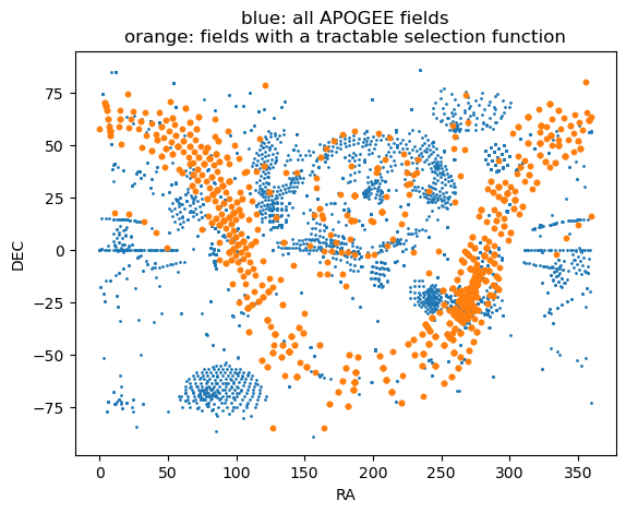
isConsistent = np.array([f in consistentField for f in designFieldNames])
plt.scatter(tDesigns["RA"], tDesigns["DEC"], s=1)
plt.scatter(tDesigns["RA"][isConsistent], tDesigns["DEC"][isConsistent], s=10)
plt.xlabel("RA")
plt.ylabel("DEC")
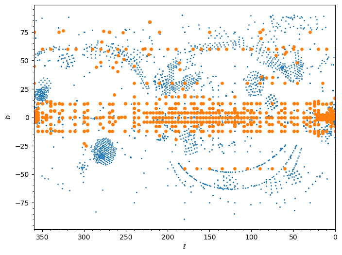
plt.title("blue: all APOGEE fields\norange: fields with a tractable selection function")
from astropy.coordinates import SkyCoord
coords = SkyCoord(tDesigns["RA"], tDesigns["DEC"], unit="deg")
plt.figure(figsize=(8, 6))
plt.scatter(coords.galactic.l, coords.galactic.b, s=1)
plt.scatter(
coords.galactic.l.value[isConsistent], coords.galactic.b.value[isConsistent], s=15
)
plt.xlabel(r"$\ell$")
plt.ylabel("$b$")
plt.xlim(360, 0)
plt.minorticks_on()
We found 71 fields with inconsistent designs.
495 of our fields have consistent designs and therefore a tractable selection function.
The selection function inside each field#
The full list of 2MASS targets inside each field is available in the following directories:
https://data.sdss.org/sas/dr17/apogee/target/apogeeObject/
https://data.sdss.org/sas/dr17/apogee/target/apogee2Object/
The binning in colour and magnitude used for target selection is given in the allDesign table:
https://data.sdss.org/sas/dr17/apogee/target/allDesign.fits
The list of targets with succesful observations is available at:
https://data.sdss.org/sas/dr17/apogee/spectro/aspcap/dr17/synspec_rev1/allStar-dr17-synspec_rev1.fits
For each field we will:
read the entire list of available 2MASS targets
read the design from the allDesign table
compare the number of available sources in each bin to the number of sources actually observed
The Main Red Star Sample can be conveniently identified using the EXTRATARG bitmask in the allStar file. If no bits are set in EXTRATARG (i.e., EXTRATARG==0), that target meets the criteria for the Main Red Star Sample for its sky location (disk, bulge, or halo).
# only keep the main red star sample:
tAllstars = tAllstars[tAllstars["EXTRATARG"] == 0]
# with succesful observations:
hasValidRV = np.array(
    [True if foo > -1000 else False for foo in tAllstars["VHELIO_AVG"]]
)
tAllstars = tAllstars[hasValidRV]
# remove trailing spaces in their field names:
observedNames = np.array([n.strip() for n in tAllstars["FIELD"]])
This downloads the 2MASS data directly from the SDSS page. For field 034-06 the file is about 100 MB.
Alternatively, download the file separately and read from the location on your drive.
%%time
example_field = '034-06'
#tField = Table.read(f"https://data.sdss.org/sas/dr17/apogee/target/apogee2Object/apogee2Object_{example_field}.fits")
tField = Table.read(f"/home/brown/Gaia/GaiaUnlimited/APOGEE/apogee2Object_{example_field}.fits")
CPU times: user 202 ms, sys: 17 ms, total: 219 ms
Wall time: 219 ms
thisDesign = tDesigns[designFieldNames == example_field][0]
print("The H and (J-K)_0 bins used to select targets in this field are:\n")
print("COHORT_MIN_H", thisDesign["COHORT_MIN_H"])
print("COHORT_MAX_H", thisDesign["COHORT_MAX_H"])
print("BIN_DEREDDENED_MIN_JK_COLOR", thisDesign["BIN_DEREDDENED_MIN_JK_COLOR"])
print("BIN_DEREDDENED_MAX_JK_COLOR", thisDesign["BIN_DEREDDENED_MAX_JK_COLOR"])

deReddenedJK = tField["J"] - tField["K"] - 1.5000 * tField["AK_TARG"]
obs_JK = (
    tAllstars["J"][observedNames == example_field]
    - tAllstars["K"][observedNames == example_field]
)
obs_deReddenedJK = (
    obs_JK - 1.5000 * tAllstars["AK_TARG"][observedNames == example_field]
)
obsH = tAllstars["H"][observedNames == example_field]


plt.figure()

plt.title("APOGEE-2 field\n%s" % (example_field))

plt.scatter(deReddenedJK, tField["H"], s=1, c="#bbbbbb", rasterized=True)
plt.scatter(-1, -1, s=3, c="#aaaaaa", label="available sources\n(2MASS)")
plt.scatter(obs_deReddenedJK, obsH, c="firebrick", s=10, label="APOGEE DR17")

# limits:
plt.xlim(0.3, 1.15)
plt.ylim(13.5, 6.5)
# add design grid:
plt.plot(
    [0.5, max(obs_deReddenedJK) + 0.1],
    [thisDesign["COHORT_MIN_H"][0], thisDesign["COHORT_MIN_H"][0]],
    "k--",
    lw=1,
)
plt.plot(
    [0.5, max(obs_deReddenedJK) + 0.1],
    [thisDesign["COHORT_MAX_H"][0], thisDesign["COHORT_MAX_H"][0]],
    "k--",
    lw=1,
)
#
plt.plot(
    [0.5, max(obs_deReddenedJK) + 0.1],
    [thisDesign["COHORT_MIN_H"][1], thisDesign["COHORT_MIN_H"][1]],
    "k--",
    lw=1,
)
plt.plot(
    [0.5, max(obs_deReddenedJK) + 0.1],
    [thisDesign["COHORT_MAX_H"][1], thisDesign["COHORT_MAX_H"][1]],
    "k--",
    lw=1,
)
#
plt.plot(
    [0.5, max(obs_deReddenedJK) + 0.1],
    [thisDesign["COHORT_MIN_H"][2], thisDesign["COHORT_MIN_H"][2]],
    "k--",
    lw=1,
)
plt.plot(
    [0.5, max(obs_deReddenedJK) + 0.1],
    [thisDesign["COHORT_MAX_H"][2], thisDesign["COHORT_MAX_H"][2]],
    "k--",
    lw=1,
)
# and colour bin:
plt.plot(
    [
        thisDesign["BIN_DEREDDENED_MIN_JK_COLOR"][0],
        thisDesign["BIN_DEREDDENED_MIN_JK_COLOR"][0],
    ],
    [min(thisDesign["COHORT_MIN_H"]), max(thisDesign["COHORT_MAX_H"])],
    "k--",
    lw=1,
)
plt.plot(
    [
        thisDesign["BIN_DEREDDENED_MIN_JK_COLOR"][1],
        thisDesign["BIN_DEREDDENED_MIN_JK_COLOR"][1],
    ],
    [min(thisDesign["COHORT_MIN_H"]), max(thisDesign["COHORT_MAX_H"])],
    "k--",
    lw=1,
)
#
plt.xlabel("$(J-K_s)_0 = J - K_s - 1.5 \\times A_K$")
plt.ylabel("$H$")
plt.minorticks_on()

plt.text(
    0.48, 13.2, "long", fontsize=13, color="k", rotation=0, horizontalalignment="right"
)
plt.text(
    0.48,
    12.65,
    "medium",
    fontsize=13,
    color="k",
    rotation=0,
    horizontalalignment="right",
)
plt.text(
    0.48,
    11.35,
    "short",
    fontsize=13,
    color="k",
    rotation=0,
    horizontalalignment="right",
)
plt.text(0.6, 9.85, "blue", fontsize=13, color="k")
plt.text(0.9, 9.85, "red", fontsize=13, color="k")

plt.legend(framealpha=1)
The H and (J-K)_0 bins used to select targets in this field are:

COHORT_MIN_H [10.0 12.199999809265137 12.800000190734863]
COHORT_MAX_H [12.199999809265137 12.800000190734863 13.300000190734863]
BIN_DEREDDENED_MIN_JK_COLOR [0.5 0.800000011920929 999.0 999.0 999.0]
BIN_DEREDDENED_MAX_JK_COLOR [8.00e-01 9.99e+02 9.99e+02 9.99e+02 9.99e+02]
<matplotlib.legend.Legend at 0x7fb9f4821640>
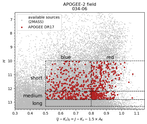
The selection function in each region of the colour-magnitude diagram and in each field is then simply obtained as the ratio of APOGEE DR17 stars (red points) to the number of available 2MASS stars (grey points).